Climate and Sustainability
General Insurance
Return of the Damned Child: Understanding ENSO in a Changing Climate




Claim your CPD points
The El Niño Southern Oscillation (“ENSO”) was formally identified in the 1920s by Sir Gilbert Walker (who observed the Southern Oscillation see-saw atmospheric pressure component across the equatorial Pacific Ocean) and later, Jacob Bjerknes (who linked ocean currents to the said see-saw atmospheric pressure oscillation). Long before this, Peruvian fishermen had already named the phenomenon 'El Niño' (for Christ Child) to describe occasional poor fish harvests that occur leading up to Christmas due to the arrival of warm, nutrient-poor ocean currents.
Since its discovery, ENSO has become one of the world's most studied climate phenomena because it is predictable months in advance, persistent and exerts far-reaching direct and indirect impacts on global climate. ENSO has three phases: El Niño, La Niña and Neutral. In general, during El Niño, Australia is more likely to experience warmer and drier conditions, increasing the risk of drought and bushfires. During La Niña, warmer ocean waters near Australia typically bring higher rainfall, greater flood risk and more tropical cyclone activity. With respect to global agricultural productivity, although not as severe as the global famine of the late 1800s (where millions perished during a large El Niño event), some regions continue to experience food security and heightened conflict risk concerns. Regional economic impacts have also been felt. For example, in Australia, insurance claims costs are typically elevated during La Niña years, as evidenced by the 2022 East Coast Floods, which resulted in over AUD 6bn in insured losses.
Despite decades of intensive research and major advances in seasonal forecasting, many aspects of ENSO remain poorly understood. This includes how each event differs from previous ones, the mechanisms driving extreme events, decadal variations, ENSO’s influence on a range of climate variables, and more recently, how ENSO will evolve under background warming due to climate change. Reputable global forecasting agencies such as the National Oceanic and Atmospheric Administration (NOAA), Copernicus members and Bureau of Meteorology (BoM) have recently declaring the event, with abundant commentary warning of a 'Super El Niño' In this context, we attempt to bring some clarity in this noisy space by critically evaluating the uncertainties inherent in the prediction of ENSO, its impacts on key regional climate variables such as temperature and rainfall, and how global warming is already changing and expected to further change key characteristics of ENSO.
It can be confusing when some meteorological agencies declare an El Niño while others do not. This arises because, while agencies are aligned on the fundamental physics of the phenomenon itself [1] , they may disagree on the timing and strength of each event. This may be due to different Sea Surface Temperature (SST) thresholds and treatment of atmospheric coupling [2] .
Beyond declaration, the timing and strength of ENSO events are predicted using statistical and dynamical models. In short, statistical models forecast ENSO by identifying historical relationships between predictors (such as current SSTAs, trade wind strength, and previous ENSO states) and associated lagged outcomes. Statistical models can be broadly divided into two types - one that works based on historical transition probabilities (i.e., "what are the odds of two El Niños in a row"), focused on lead times longer than 12 months, and the other shorter-term type that focuses on current observations of predictor variables. These models are relatively easy to run, and possess reasonable skill, although they are constrained to predicting events that have historical analogs.
On the other hand, dynamical models are computationally expensive as they explicitly solve the governing equations and try to essentially replicate (simplified) ocean and atmospheric interactions such as ocean currents, heat transport, convective processes and Kelvin/Rossby waves*. The results from these models are typically most informative for seasonal forecasts from three to six month lead times. Ensembles of dynamic models are increasingly used in order to obtain a range of possible future climate outcomes spanning months out to a year. This means that the potential impacts can be more confidently detected and a range of alternate future climate states identified. The skill of the models varies seasonally and also regionally.
| Model Class | Subtype | Core Approach | Lead Time Range |
| Dynamical models | - | Simulate atmospheric, oceanic, and land-surface processes by solving physical equations governing the climate system. | Days to months |
| Statistical models | Historical transition probability | Estimate the probability of transitions between climate states from historical observations (e.g., Markov chains, empirical transition matrices). | 12 months |
| Statistical models | Seasonal prediction | Use empirical relationships between climate predictors and seasonal outcomes through regression, analogue methods, or machine learning. | 1-6 months |
A prediction can only be considered valuable if it yields accuracy greater than a coin toss (> 50%). In general, both breeds of models - particularly dynamical models - naturally improve in accuracy with shorter lead times. However, forecast skill drops dramatically when forecasts pass through the March-May period, meaning that a forecast issued in January for July has poor skill compared to one issued in July for December. This well-known challenge in ENSO prediction is commonly referred to as the 'April or (Boreal) Spring Predictability Barrier'. This is because the March-May period it is a season where feedbacks are weakest and seasonal noise is strongest - meaning that a single wind burst or tropical cyclone may determine whether an ENSO event develops. Although recent advances in data capture and assimilation, higher model resolution, ensemble forecasting and AI have improved model performance, the spring predictability barrier has not been truly overcome to date.
Instructively, that the 2014 Super El Niño event failed prediction provides a timely reminder of the limits of modern ENSO forecasting. In early 2014, ocean temperatures looked remarkably similar to previous major events such as the 1982 and 1997 El Niños, with many models, as early as March, projecting anomalies exceeding +2 deg C by July. However, the 'handshake' between ocean and atmosphere failed to materialize. The lack of reinforcing westerly wind bursts stalled the amplification of early signs of warming and resulted in a borderline weak El Niño/ Neutral event. Instead, the initial build-up of excess ocean heat lingered around long enough and contributed to the most recent extreme El Niño event the very next year in 2015.
Impacts of ENSO on seasonal rainfall, flood and bushfire risk have generally been well documented in scientific literature. As such, this section will not provide an exhaustive review but instead attempt to dispel common misconceptions by highlighting key nuances. These include maximum impact periods, degree of influence according to different ENSO 'flavours', variable types and interaction with different climate modes such as the Indian Ocean Dipole (IOD).
Firstly, ENSO events are often blamed for causing heatwaves, floods, fires and typhoons. This sweeping statement effectively masks two critical nuances: that there is an upper limit to ENSO's impact on variables (often expressed as 'variance explained') as well as the strength of influence over a range of variables. ENSO has the most direct effect on regional ocean temperatures, seasonal rainfall totals and surface air average temperatures. ENSO is also related to flood and bushfire risk, but with a far higher signal-to-noise ratio (for example, bushfire risk also depends on rainfall conditions in the previous years). Perhaps most instructively, tropical cyclone risk is only tenuously associated with ENSO due to counter-acting effects on vertical wind shear, SST and high hit-miss-component with landfalls. A famous example is the 1992 Hurricane season with only seven named storms (associated with El Niño) versus an average of 14, yet it produced one of the insurance industry's largest losses at that time with Hurricane Andrew.
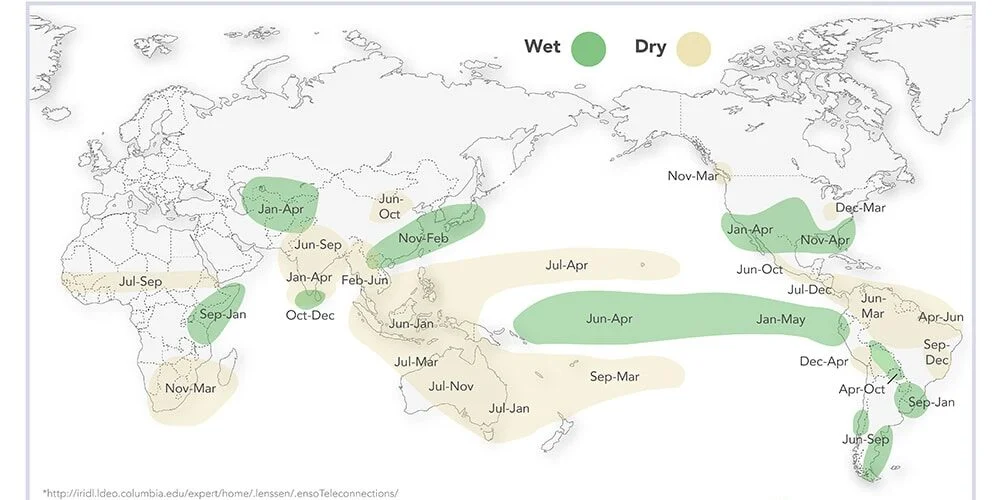
Figure 1: Typical rainfall impacts associated with El Niño. Source: International Research Institute for Climate and Society (IRI), Columbia University
Another common misconception is the assumption that regional impacts of ENSO always occur simultaneously with the peak of SST anomalies. Instead, across the Asia Pacific region, both rainfall and temperature often show a range of delayed or 'lagged' response. This is because ENSO affects large scale circulation (i.e., monsoon, subtropical highs, land-atmosphere feedbacks) rather than direct forcing. For example, in East Australia and Indonesia, impacts of ENSO on rainfall often occur in September-October-November (SON) due to being triggered more directly. However, across South East Asian countries that flank the Northwest Pacific basin, rainfall is dominated by the Southwest Monsoon and hence ENSO may have a lagged impact the next May - October. Another example of atmospheric 'memory' of ENSO is evidenced through more severe temperature anomalies in the year following the event due to reduced soil moisture (due to reduced rainfall and increased evaporation due to reduced cloud cover) and a key reason why researchers often focus on impacts in the ENSO 'decay' year rather than at its peak.
The strength of rainfall and other impacts are determined not just by the strength of the ENSO event alone, but by the type of ENSO event (not all El Niños are equal), and the interaction of ENSO with other climate modes. Broadly speaking, El Niño events can be divided into Eastern Pacific (canonical/ classic) El Niños and Central Pacific or Modoki (coined by Japanese research Prof. Yamagata who first observed the phenomenon) events - these events are characterised by where maximum SSTAs are observed. For example, eastern Australia experienced more significant rainfall anomalies during 2004-5, 2019 Modoki events versus the 97-98 event or 15-16 large East Pacific events. This shows that 'textbook' El Niños do not tell the whole story, and that there is high sensitivity to the exact location of the SST anomalies and ultimate impacts. Similarly, the impacts of ENSO can be exacerbated if they coincide with other climate modes. A famous instance was the 2010-11 La Niña event that caused widespread flooding events from Brisbane to Thailand. At that time, a strong La Niña coincided with a negative IOD event, which exacerbated the atmospheric response.
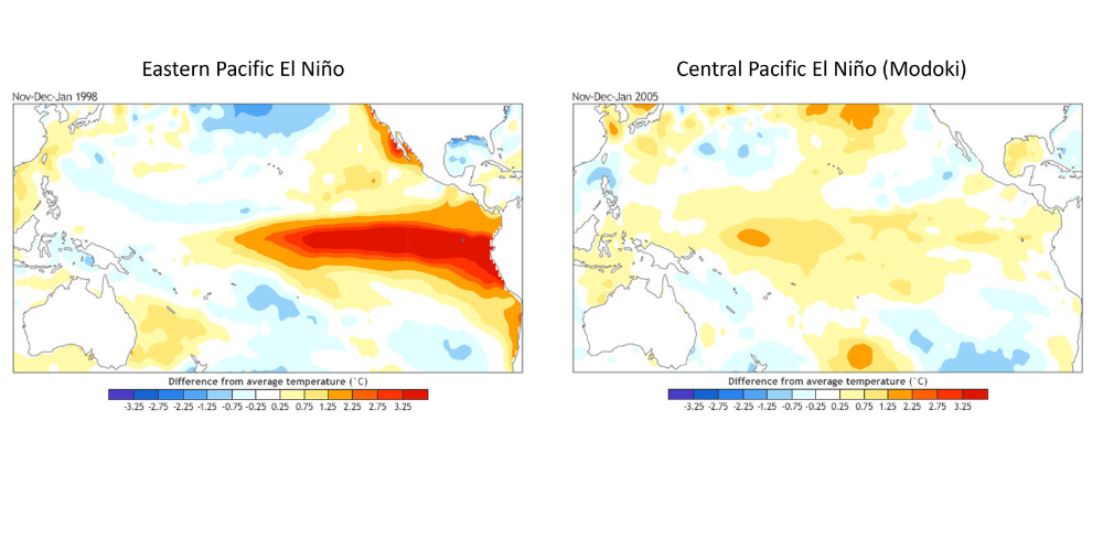
Figure 2: The difference between a Central Pacific and Eastern Pacific El Niño. Source: https://www.climate.gov/news-features/blogs/enso/enso-flavor-month
Understanding how ENSO is declared, predicted and felt is only half the picture. Part Two of this series turns to how climate change is already reshaping ENSO, and what the current El Niño event means for the Asia-Pacific region through to December 2026. Read Part Two: How Is Climate Change Reshaping ENSO?
References
[1] El Niños, in essence, represent persistent warm Sea Surface Temperature Anomaly (SSTA) in the East Equatorial Pacific Region, coupled with a weakening or reversing (in extreme cases) of elements of the Walker Circulation and associated westerly winds.
[2] For example, NOAA often identifies El Niños earlier as it uses a lower threshold (+0.5°C) compared to the BoM (+0.8°C) for five overlapping three-month periods within the Niño 3.4 region. On the other hand, the Japanese Meteorological Agency (JMA) monitors anomalies across slightly different regions of the ocean that persist for more than six months. Importantly, despite these nuances, all agencies have a focus on other atmospheric clues that El Niño has formed through weakened trade wind activity, altered deep convection patterns and sea level pressure changes.
The views expressed in this article are those of the author(s) or working group named below, and do not necessarily reflect the views of the Actuaries Institute. This work is licensed under a Creative Commons Attribution-NonCommercial-No Derivatives CC BY-NC-ND Version 4.0.


From physical risk modelling to transition pathways, explore our latest thinking on climate and sustainability
Subscribe to Actuaries Digital for free and receive the latest actuarial analysis, research, and commentary direct to your inbox